My Secret Rainbow

XAI进行到底 —PDP&ICE图（三）

1 部分依赖图（Partial Dependence Plot)

1.1 理论解读

参考：「AI黑箱探测」事后模型归因解析Part 1

部分依赖图简称PDP图，能够展现出一个或两个特征变量对模型预测结果影响的函数关系：近似线性关系、单调关系或者更复杂的关系。

单一变量PDP图的具体实施步骤如下：

• 挑选一个我们感兴趣的特征变量，并定义搜索网格；
• 将搜索网格中的每一个数值代入上述PDP函数中的X_s，使用黑箱模型进行预测，并将得到的预测值取平均；
• 画出特征变量的不同取值与预测值之间的关系，该图即为部分依赖图。

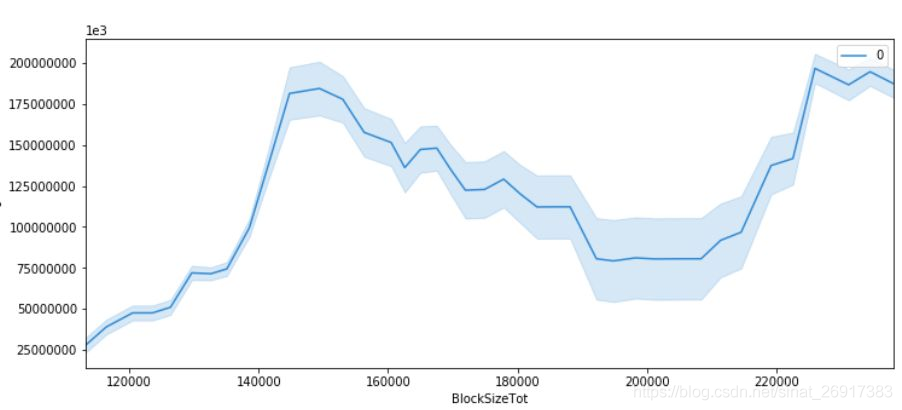
以比特币数据集为例，我们使用PDP方法对Xgboost模型结果进行解析。下图刻画的是单变量“区块大小”与比特币价格之间的函数关系。这是一个典型的非线性关系：当“区块大小”在12000-15000范围内增长时，比特币价格逐渐上涨；随着“区块大小”的进一步增长，会对比特币价格产生负向影响，直到区块大小高于20000时，又会对比特币价格产生正向影响。

PDP图的优点在于易实施，缺点在于不能反映特征变量本身的分布情况，且拥有苛刻的假设条件——变量之间严格独立。若变量之间存在相关关系，会导致计算过程中产生过多的无效样本，估计出的值比实际偏高。另一个缺点是样本整体的非均匀效应（Heterogeneous effect）：PDP只能反映特征变量的平均水平，忽视了数据异质对结果产生的影响。

1.2 如何根据PDP 进行特征筛选

PDP, ICE: 模型可视化技术之一

特征选择：

• 当某个特征的PDP曲线几乎水平或者无规律抖动的时候, 这个特征可能是无用的特征.
• 当某个特征的PDP曲线非常陡峭的时候, 说明这个特征的贡献度是比较大的.

---

2 个体条件期望图（Individual Conditional Expectation Plot)

参考：「AI黑箱探测」事后模型归因解析Part 1

个体条件期望图（ICE Plot）计算方法与PDP类似，它刻画的是每个个体的预测值与单一变量之间的关系。个体条件期望图消除了非均匀效应的影响，它的原理和实现方法如下：对某一个体，保持其他变量不变，随机置换我们选定的特征变量的取值，放入黑箱模型输出预测结果，最后绘制出针对这个个体的单一特征变量与预测值之间的关系图。

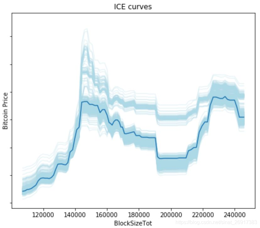
继续以上述比特币数据为例，下图反映的是“区块大小”对比特币价格影响的ICE图，其中浅蓝色线反映的是每个个体的条件期望图，深蓝色线反映所有个体的平均水平。从图中可看出所有个体并不一定遵循相同的变化趋势，因此相较于PDP的一概而论，ICE图能够更准确地反映特征变量与目标之间的关系。

ICE图的优点在于易于理解，能够避免数据异质的问题。在ICE图提出之后，人们又提出了衍生ICE图，能够进一步检测变量之间的交互关系并在ICE图中反映出来。

ICE图的缺点在于只能反映单一特征变量与目标之间的关系，仍然受制于变量独立假设的要求，同时ICE图像往往由于个体过多导致图像看起来过于冗杂，不容易获取解释信息。

---

3 sklearn 0.24+实现：PDP&ICE图

sklearn 0.24版本有更新两个图的画法，可参考：Partial Dependence and Individual Conditional Expectation Plots

3.1 部分依赖图（Partial Dependence Plot)

print('Computing partial dependence plots...')
tic = time()
features = ['MedInc', 'AveOccup', 'HouseAge', 'AveRooms']
display = plot_partial_dependence(
       est, X_train, features, kind="average", subsample=50,
       n_jobs=3, grid_resolution=20, random_state=0
)
# average / individual 

print(f"done in {time() - tic:.3f}s")
display.figure_.suptitle(
    'Partial Dependence Plot\n'
)
display.figure_.subplots_adjust(hspace=0.3)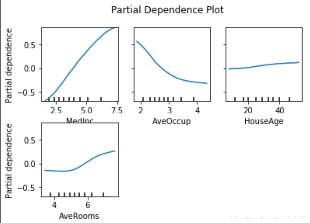

3.2 二维-部分依赖图（Partial Dependence Plot)

features = ['AveOccup', 'HouseAge', ('AveOccup', 'HouseAge')]
print('Computing partial dependence plots...')
tic = time()
_, ax = plt.subplots(ncols=3, figsize=(9, 4))
display = plot_partial_dependence(
    est, X_train, features, kind='average', n_jobs=3, grid_resolution=20,
    ax=ax,
)
print(f"done in {time() - tic:.3f}s")
display.figure_.suptitle(
    'Partial dependence of house value on non-location features\n'
    'for the California housing dataset, with Gradient Boosting'
)
display.figure_.subplots_adjust(wspace=0.4, hspace=0.3)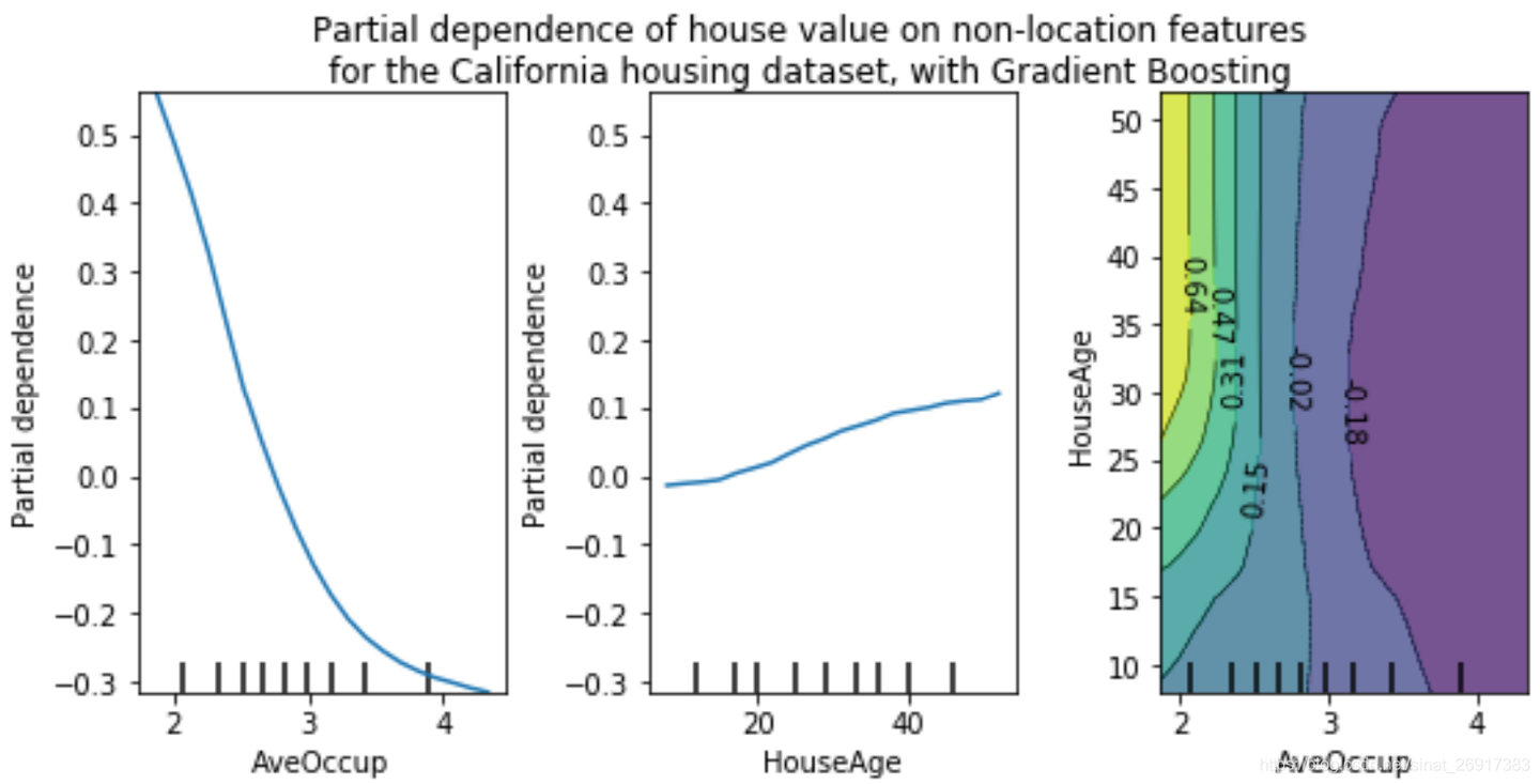

3.3 Individual Conditional Expectation Plot

个体条件期望图（Individual Conditional Expectation Plot)

print('Computing partial dependence plots...')
tic = time()
features = ['MedInc', 'AveOccup', 'HouseAge', 'AveRooms']
display = plot_partial_dependence(
       est, X_train, features, kind="individual", subsample=50,
       n_jobs=3, grid_resolution=20, random_state=0
)
# average / individual 

print(f"done in {time() - tic:.3f}s")
display.figure_.suptitle(
    'Individual Conditional Expectation Plot\n'
)
display.figure_.subplots_adjust(hspace=0.3)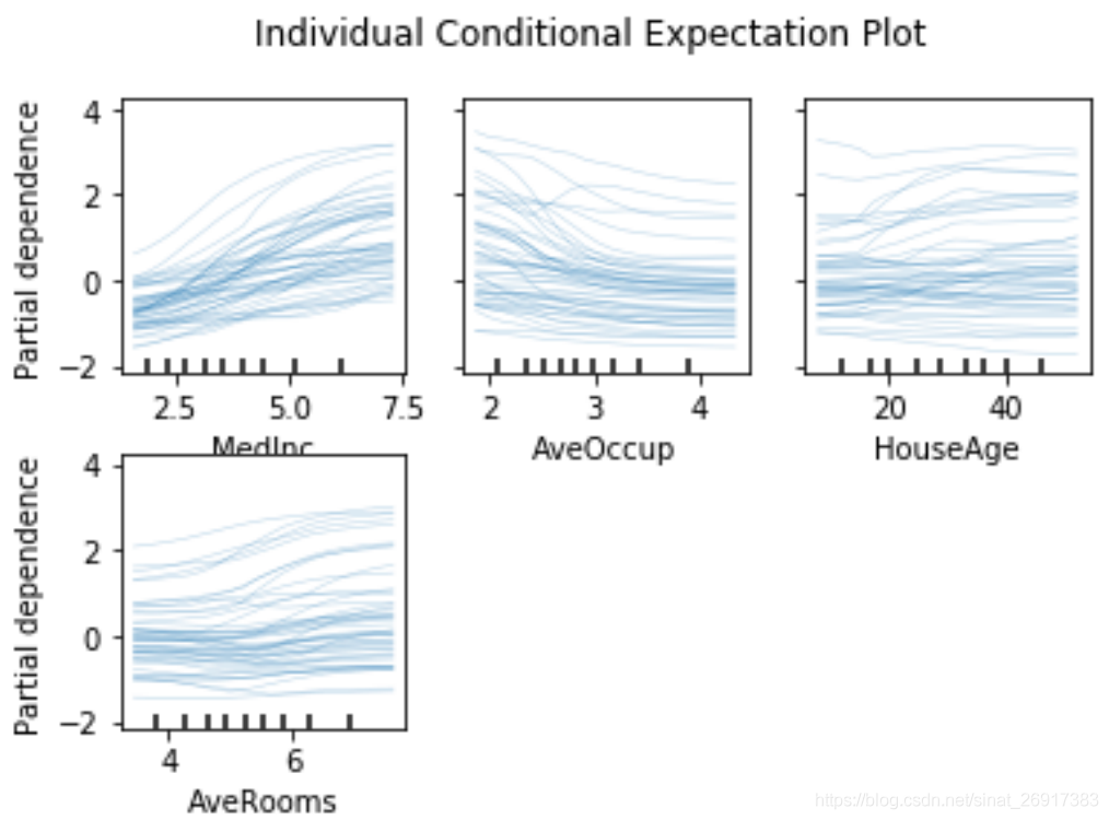

3.4 both:PDP + ICE

# both = PDP + ICE
print('Computing partial dependence plots...')
tic = time()
features = ['MedInc', 'AveOccup', 'HouseAge', 'AveRooms']
display = plot_partial_dependence(
       est, X_train, features, kind="both", subsample=50,
       n_jobs=3, grid_resolution=20, random_state=0
)
# average / individual 

print(f"done in {time() - tic:.3f}s")
display.figure_.suptitle(
    'Individual Conditional Expectation Plot\n'
)
display.figure_.subplots_adjust(hspace=0.3)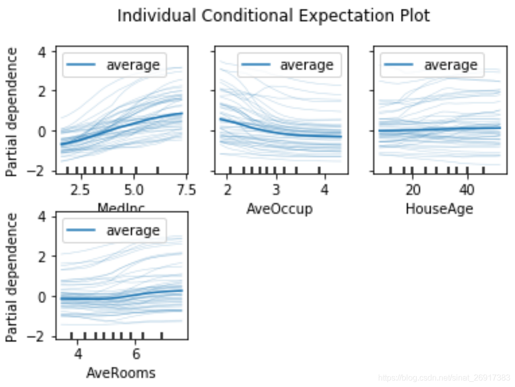

其中，深色的是PDP，浅色的是ICE的样本

原文：https://zhuanlan.zhihu.com/p/364921771